Take your reporting capabilities to the next level with the introduction of Excel pivot tables in Acumatica 6. Pivot tables are one of the key business intelligence tools in Excel, and now you can create and share them within Acumatica without the extra steps of exporting or importing your data.
3 Main Parts of a Pivot Table:
- Source or raw data you want to analyze.
- Design a pivot table based on the data.
- Use the pivot table and the visualization tools to gather valuable business information.
Why use pivot tables?
- You have access to 100% of your data. All of your company’s data from the Organization, Projects, Finance, and Distribution modules is exposed as a data source through Generic Inquiries (GI) using Data Access Classes (DAC).
- The values in the pivot table provide drill-down capability to the detail documents that are the source of the data.
- Access rights to pivot tables are managed through the standard Acumatica role based security module
In Acumatica, the same parts of a pivot table apply:
- Use an existing (or create a new) Generic Inquiry from the Site Map to use as a raw data source
- Design a pivot table based on the Generic Inquiry
- Share the pivot table to all authorized users and let them use the data visualization tools in order to turn raw data into useful business information
Example: Pivot Table to analyze sales performance measures
We are going to create a pivot table to analyze sales performance of Sales Persons per quarter.
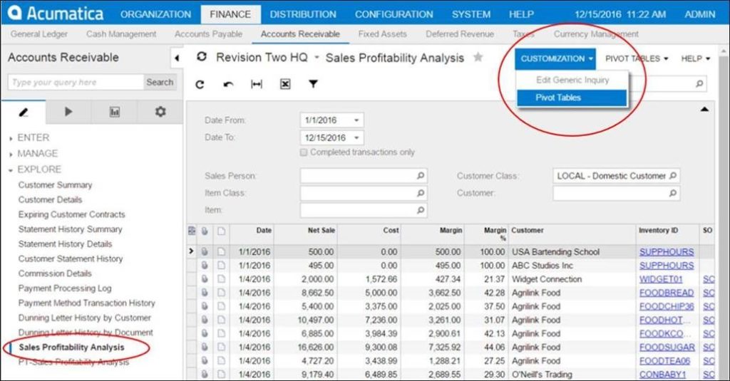
- Select the Sales Profitability Analysis Generic Inquiry from the A/R>EXPLORE menu. This GI provides the source data that we need.
- Start the pivot table design by selecting Pivot Tables from the CUSTOMIZATION menu in the GI.

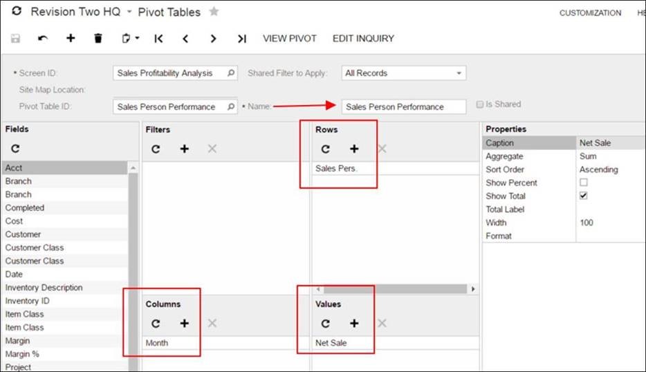
- Acumatica takes you to the Pivot Table design page with the GI name preselected in the Screen ID field. This is the actual screen (SM208010) for all pivot tables in the system: SYSTEM>Customization>Pivot Tables
- Click the plus sign to add a new pivot table to the GI and get a clean slate. Notice that the Fields pane is filled with the names of the GI columns. Just drag and drop these fields to one of four possible destination panes (Filters, Rows, Columns, or Values) in order to create your pivot table.

- We will start by creating a simple pivot table that shows the powerful capabilities provided by the tool.
Type a name in the Name field and click the save button.
Drag and drop these 3 fields from the Fields pane:
Sales Pers. Field to the Rows pane
Month field to the Columns pane
Net Sale field to the Values pane
- Click the VIEW PIVOT button to display the pivot table.
Comments:
- The Sales Pers. field was selected as Rows, and it is retrieving the list of all names available from the data source.
- The Month field, selected as Columns, dynamically created one column for each available month in the data.
- The Net Sales field provided the values for each Sales Person and Month. Notice in the previous screen that we used the default Aggregate of SUM.
- Each aggregated value in the cells is a hyperlink that allows you to drill down to the actual transactions that provided the data.
- Note: click the value of $3,900 for Jason Mendenhall under 01-2016 to display the underlying orders. From there, you can keep drilling down to the order detail.
- You can sort aggregated data.
- Note: you can also sort the right-most column of Totals in descending order to instantly identify your top performers.

- Note: you can also sort the right-most column of Totals in descending order to instantly identify your top performers.
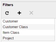
7. Go back to the pivot table – drag and drop some fields to the Filters pane.

8. Click the VIEW PIVOT to display the pivot table.
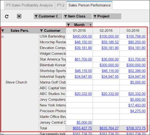
9. Drag and drop the Customer field from the filters section to the Rows section, right of the Sales
Pers. field.

The Customers are now grouped by Sales Person, which gives you full visibility of their sales and
the ability to drill down to the specific orders.

Want to know more about Pivot Tables in Acumatica 6:
Here are a couple useful links:
If you have questions or need some assistance, visit our support page for more help.